Polynomial Regression in Machine Learning

In real-world Machine Learning problems, data does not always follow a straight-line pattern. While Linear Regression works well when the relationship between variables is approximately linear, it can struggle when the data contains curves and other non-linear patterns.

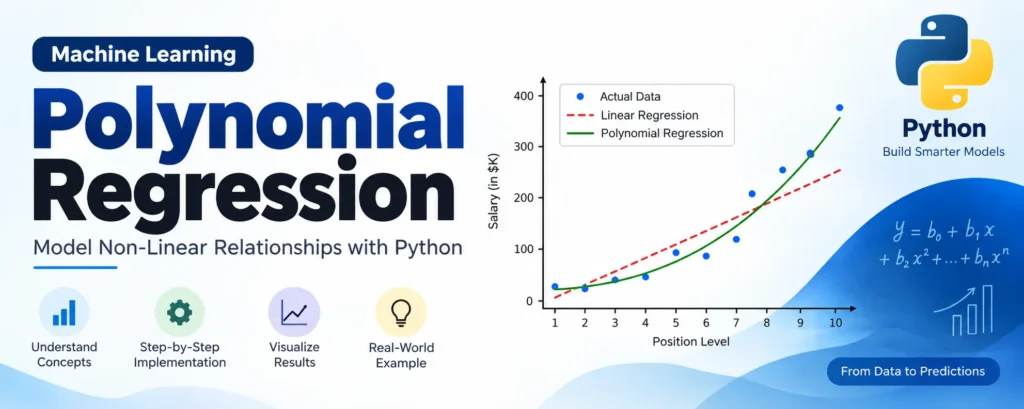
This is where Polynomial Regression becomes useful. Polynomial Regression extends Linear Regression by adding higher-degree terms such as x², x³, and x⁴ to capture non-linear relationships between input and output variables.

In this article, we will understand Polynomial Regression in Machine Learning, its formula, how it works, the difference between Linear and Polynomial Regression, and how to implement it in Python using a practical salary prediction example.

Complete Advance AI Topics: Click Here
SQL Tutorial: Click Here

What is Polynomial Regression?

Polynomial Regression is a supervised Machine Learning algorithm used to model a non-linear relationship between an independent variable and a dependent variable.

The general polynomial regression equation is:

y = b₀ + b₁x + b₂x² + b₃x³ + … + bₙxⁿ

Where:

y = predicted output
x = input feature
b₀ = intercept
b₁, b₂, …, bₙ = model coefficients
n = degree of the polynomial

For example, a second-degree polynomial can be written as:

y = b₀ + b₁x + b₂x²

A fourth-degree polynomial would be:

y = b₀ + b₁x + b₂x² + b₃x³ + b₄x⁴

Why is Polynomial Regression Considered a Linear Model?

Although Polynomial Regression produces a curved prediction line, it is still considered a linear regression model because the model is linear with respect to its coefficients.

For example:

y = b₀ + b₁x + b₂x²

The input contains powers of x, but the coefficients b₀, b₁, and b₂ are still combined linearly.

This allows us to use Linear Regression after transforming the original features into polynomial features.

Polynomial Regression vs Linear Regression

The main difference is the type of relationship each model is designed to capture.

Feature	Linear Regression	Polynomial Regression
Relationship	Approximately linear	Non-linear or curved
Equation	y = b₀ + b₁x	y = b₀ + b₁x + b₂x² + …
Prediction Shape	Straight line	Curve
Feature Transformation	Not required	Polynomial features are created
Model Complexity	Lower	Depends on polynomial degree

Why Do We Need Polynomial Regression?

Linear Regression assumes that the relationship between the input and output can be represented reasonably well by a straight line.

However, many real-world datasets contain non-linear relationships. For example:

Salary may increase rapidly at higher job levels.
Sales may follow a curved growth pattern.
Temperature and energy consumption may have non-linear relationships.
Product demand can change differently at different price levels.

If we use a straight line for strongly curved data, the model may produce large prediction errors.

Polynomial Regression solves this problem by introducing additional polynomial terms that allow the model to fit a curve.

How Does Polynomial Regression Work?

Polynomial Regression generally works in two major steps:

Transform the original features into polynomial features.
Train a Linear Regression model using those transformed features.

For example, if our original feature is:

x

Polynomial transformation with degree 3 creates:

1, x, x², x³

The Linear Regression model can then learn the coefficients for these transformed features.

Polynomial Regression converts the original feature space into a higher-dimensional polynomial feature space and then applies Linear Regression.

Understanding Polynomial Degree

The degree determines how complex the polynomial curve can become.

Degree 1: Equivalent to Linear Regression.
Degree 2: Produces a quadratic curve.
Degree 3: Produces a cubic curve.
Degree 4: Can capture more complex curves.
Very high degree: Can lead to overfitting.

Increasing the degree does not automatically make a model better. A very high-degree polynomial can fit the training data extremely well while performing poorly on unseen data.

Real-World Example: Salary Prediction

Let’s understand Polynomial Regression with a practical example.

Suppose a company is hiring a candidate who claims that their previous salary was $160,000 per year.

The HR department has salary information for employees at different position levels. Because salary does not increase at a constant rate across all levels, we can use Polynomial Regression to estimate the expected salary for a particular level.

Our goal is to predict the salary for position level 6.5 and compare the result with the candidate’s claimed salary.

Step-by-Step Implementation of Polynomial Regression in Python

Step 1: Import Libraries and Load Dataset

import numpy as np
import pandas as pd
import matplotlib.pyplot as plt

# Load dataset
dataset = pd.read_csv('Position_Salaries.csv')

# Extract position level and salary
X = dataset.iloc[:, 1:2].values
y = dataset.iloc[:, 2].values

Here, X contains the position levels and y contains the corresponding salaries.

The position name is not used for prediction because it is descriptive information. The numerical Level column is used as the input feature.

Step 2: Train a Linear Regression Model

from sklearn.linear_model import LinearRegression

lin_reg = LinearRegression()
lin_reg.fit(X, y)

This Linear Regression model provides a baseline that we can compare against the Polynomial Regression model.

Step 3: Create Polynomial Features

from sklearn.preprocessing import PolynomialFeatures

poly_features = PolynomialFeatures(degree=4)

X_poly = poly_features.fit_transform(X)

The PolynomialFeatures class creates additional features based on powers of the original feature.

For example, with degree 4, the transformed data contains:

1, x, x², x³, x⁴

Step 4: Train the Polynomial Regression Model

poly_reg = LinearRegression()

poly_reg.fit(X_poly, y)

Now the Linear Regression algorithm is trained on the polynomial-transformed features.

Visualizing Linear Regression Results

We can visualize the Linear Regression model to see how well a straight line fits the salary data.

plt.scatter(X, y)
plt.plot(X, lin_reg.predict(X))

plt.title("Linear Regression - Salary Prediction")
plt.xlabel("Position Level")
plt.ylabel("Salary")

plt.show()

The resulting straight line may not represent the non-linear salary pattern accurately.

Visualizing Polynomial Regression Results

Now let’s visualize the Polynomial Regression model.

X_grid = np.arange(
    min(X),
    max(X),
    0.1
).reshape(-1, 1)

plt.scatter(X, y)
plt.plot(
    X_grid,
    poly_reg.predict(poly_features.transform(X_grid))
)

plt.title("Polynomial Regression - Salary Prediction")
plt.xlabel("Position Level")
plt.ylabel("Salary")

plt.show()

The polynomial curve can capture the non-linear relationship between position level and salary much better than a simple straight line.

Making Predictions with Linear Regression

Now let’s predict the salary for position level 6.5 using Linear Regression.

lin_pred = lin_reg.predict([[6.5]])

print("Linear Prediction:", lin_pred)

The Linear Regression model can produce a prediction that differs significantly from the actual trend in the dataset.

Making Predictions with Polynomial Regression

Let’s now use our Polynomial Regression model.

poly_pred = poly_reg.predict(
    poly_features.transform([[6.5]])
)

print("Polynomial Prediction:", poly_pred)

The polynomial model is able to capture the curved relationship in the training data and can therefore provide a prediction that better follows the observed salary pattern.

In the commonly used Position Salaries example, the degree-4 model predicts a salary close to $159K for level 6.5, which is close to the candidate’s claimed $160K salary.

Complete Polynomial Regression Code

import numpy as np
import pandas as pd
import matplotlib.pyplot as plt

from sklearn.linear_model import LinearRegression
from sklearn.preprocessing import PolynomialFeatures

# Load dataset
dataset = pd.read_csv('Position_Salaries.csv')

# Select features and target
X = dataset.iloc[:, 1:2].values
y = dataset.iloc[:, 2].values

# Linear Regression
lin_reg = LinearRegression()
lin_reg.fit(X, y)

# Polynomial Regression
poly_features = PolynomialFeatures(degree=4)
X_poly = poly_features.fit_transform(X)

poly_reg = LinearRegression()
poly_reg.fit(X_poly, y)

# Create smooth values for visualization
X_grid = np.arange(
    min(X),
    max(X),
    0.1
).reshape(-1, 1)

# Plot Polynomial Regression
plt.scatter(X, y)
plt.plot(
    X_grid,
    poly_reg.predict(poly_features.transform(X_grid))
)

plt.title("Polynomial Regression")
plt.xlabel("Position Level")
plt.ylabel("Salary")

plt.show()

# Prediction
prediction = poly_reg.predict(
    poly_features.transform([[6.5]])
)

print("Predicted Salary:", prediction)

Advantages of Polynomial Regression

Can model non-linear relationships.
Easy to implement using Python and Scikit-learn.
Works well for relatively small datasets.
Can provide a better fit than Linear Regression for curved data.
Easy to understand and visualize.

Disadvantages of Polynomial Regression

High polynomial degrees can cause overfitting.
Model complexity increases as the degree increases.
Polynomial features can become computationally expensive when there are many input features.
Predictions outside the training range can become unreliable.
The model may be sensitive to the chosen polynomial degree.

Polynomial Regression and Overfitting

One of the most important concepts to understand when using Polynomial Regression is overfitting.

If we choose a very high polynomial degree, the model may try to pass through almost every training data point. Although this can produce a very low training error, the model may fail to generalize to new data.

Therefore, instead of automatically selecting the highest possible degree, we should choose a degree that provides a good balance between underfitting and overfitting.

When Should You Use Polynomial Regression?

Polynomial Regression can be useful when:

The relationship between variables is clearly non-linear.
A straight-line model performs poorly.
The dataset is relatively small or moderate in size.
You can identify a meaningful polynomial relationship.
You need an interpretable model for a curved relationship.

Polynomial Regression Applications

Polynomial Regression can be applied to several Machine Learning and data analysis problems, including:

Salary and compensation analysis
Sales trend analysis
Demand forecasting
Temperature modeling
Performance analysis
Growth curve modeling
Economic and business trend analysis

Final Thoughts

Polynomial Regression is a useful Machine Learning technique for situations where a simple Linear Regression model cannot capture the relationship between variables.

By transforming the original features into polynomial features such as x², x³, and x⁴, we can use a Linear Regression algorithm to model curved relationships.

The most important thing to remember is that a higher polynomial degree is not always better. Choosing an appropriate degree is essential to avoid overfitting and achieve good performance on unseen data.

YT:- DecodeIT

Keywords: ML Polynomial Regression, Polynomial Regression in Machine Learning, Polynomial Regression in Machine Learning ,ML,Polynomial Regression Python, Polynomial Regression Formula, Polynomial Regression Example, Machine Learning Regression, Polynomial Regression Scikit-learn, ML Polynomial Regression Example Polynomial Regression in Machine Learning,Polynomial Regression in Machine Learning ML,ML

Polynomial Regression in Machine Learning