Naive Bayes Classifier Algorithm – A Powerful Tool for Quick and Accurate Predictions

Naïve Bayes Classifier Algorithm

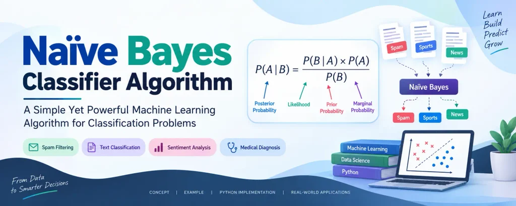
In Machine Learning, some of the simplest algorithms can produce surprisingly effective results. The Naïve Bayes Classifier is one such algorithm. It is a supervised learning algorithm based on Bayes’ Theorem and is widely used for classification problems, particularly when working with large and high-dimensional datasets such as text data.

Complete Advance AI Topics: Click Here
SQL Tutorial: Click Here

What is Naïve Bayes?

Naïve Bayes is a probabilistic classification algorithm that uses Bayes’ Theorem to predict the class of a data point based on the probability of its features. It is especially useful for classification tasks where speed and simplicity are important.

Some common applications of Naïve Bayes include:

• Spam filtering
• Sentiment analysis
• News classification

Why is it Called Naïve Bayes?

The name Naïve Bayes comes from two important concepts:

• Naïve: The algorithm assumes that the features of a dataset are independent of one another. For example, when determining whether a fruit is an apple, Naïve Bayes considers factors such as its colour, shape, and sweetness independently.
• Bayes: The algorithm is based on Bayes’ Theorem, which calculates the probability of a hypothesis based on available evidence.

Bayes’ Theorem: The Heart of Naïve Bayes

Bayes’ Theorem provides a mathematical way to update the probability of a hypothesis when new evidence becomes available.

P(A|B) = [P(B|A) × P(A)] / P(B)

Where:

• P(A|B): Posterior probability, or the probability of hypothesis A given evidence B.
• P(B|A): Likelihood, or the probability of observing B when A is true.
• P(A): Prior probability, or the initial probability of hypothesis A.
• P(B): Marginal probability, or the overall probability of observing B.

Download New Real-Time Projects: Click Here

How Naïve Bayes Works: A Practical Example

Suppose we have a dataset containing different weather conditions and information about whether a player plays or not.

Outlook	Play
Rainy	Yes
Sunny	Yes
Overcast	Yes
…	…

Now, suppose the weather forecast is Sunny. We can use Naïve Bayes to determine whether the player is likely to play.

Step 1: Create a Frequency Table

Weather	Yes	No
Overcast	5	0
Rainy	2	2
Sunny	3	2

Step 2: Calculate the Probabilities

• P(Sunny | Yes) = 3/10 = 0.3
• P(Sunny | No) = 2/4 = 0.5
• P(Yes) = 10/14 = 0.71
• P(No) = 4/14 = 0.29
• P(Sunny) = 5/14 = 0.35

Step 3: Apply Bayes’ Theorem

For the Yes class:

P(Yes | Sunny) = (0.3 × 0.71) / 0.35 ≈ 0.60

For the No class:

P(No | Sunny) = (0.5 × 0.29) / 0.35 ≈ 0.41

Since P(Yes | Sunny) > P(No | Sunny), the model predicts that the player should play when the weather is sunny.

Advantages of Naïve Bayes

• It is fast and simple to implement.
• It works efficiently with large datasets.
• It performs well for multi-class classification.
• It is particularly effective for text classification.

Disadvantages of Naïve Bayes

• It assumes that features are independent, which may not always be true in real-world datasets.
• It cannot effectively learn complex interactions between features.

Applications of Naïve Bayes

Naïve Bayes is used in a variety of real-world applications, including:

• Email spam filtering
• Medical diagnosis
• Credit scoring
• Sentiment analysis
• Real-time prediction systems

Types of Naïve Bayes Models

1. Gaussian Naïve Bayes: Assumes that the features follow a normal distribution and is commonly used for continuous data.
2. Multinomial Naïve Bayes: Commonly used for document and text classification where features represent word frequencies.
3. Bernoulli Naïve Bayes: Designed for binary or Boolean features and is useful when features represent the presence or absence of something.

Naïve Bayes Classifier in Python Step-by-Step

Let’s implement a simple Naïve Bayes classifier using the user_data.csv dataset.

Step 1: Data Pre-processing

import numpy as np
import matplotlib.pyplot as plt
import pandas as pd

# Load dataset
dataset = pd.read_csv('user_data.csv')

x = dataset.iloc[:, [2, 3]].values
y = dataset.iloc[:, 4].values

# Split data
from sklearn.model_selection import train_test_split

x_train, x_test, y_train, y_test = train_test_split(
    x, y, test_size=0.25, random_state=0
)

# Feature Scaling
from sklearn.preprocessing import StandardScaler

sc = StandardScaler()

x_train = sc.fit_transform(x_train)
x_test = sc.transform(x_test)

Step 2: Fit the Naïve Bayes Model

from sklearn.naive_bayes import GaussianNB

classifier = GaussianNB()
classifier.fit(x_train, y_train)

Step 3: Predict the Test Set

y_pred = classifier.predict(x_test)

Step 4: Generate the Confusion Matrix

A confusion matrix can be used to compare the predicted results with the actual test labels.

from sklearn.metrics import confusion_matrix

cm = confusion_matrix(y_test, y_pred)

print(cm)

YT:- DecodeIT

Step 5 & 6: Visualize the Training and Test Sets

from matplotlib.colors import ListedColormap

def visualize_set(x_set, y_set, title):
    X1, X2 = np.meshgrid(
        np.arange(
            start=x_set[:, 0].min() - 1,
            stop=x_set[:, 0].max() + 1,
            step=0.01
        ),
        np.arange(
            start=x_set[:, 1].min() - 1,
            stop=x_set[:, 1].max() + 1,
            step=0.01
        )
    )

    plt.contourf(
        X1,
        X2,
        classifier.predict(
            np.array([X1.ravel(), X2.ravel()]).T
        ).reshape(X1.shape),
        alpha=0.75,
        cmap=ListedColormap(('purple', 'green'))
    )

    plt.xlim(X1.min(), X1.max())
    plt.ylim(X2.min(), X2.max())

    for i, j in enumerate(np.unique(y_set)):
        plt.scatter(
            x_set[y_set == j, 0],
            x_set[y_set == j, 1],
            c=ListedColormap(('purple', 'green'))(i),
            label=j
        )

    plt.title(title)
    plt.xlabel('Age')
    plt.ylabel('Estimated Salary')
    plt.legend()
    plt.show()


# Visualize Training Set
visualize_set(
    x_train,
    y_train,
    'Naive Bayes (Training set)'
)

# Visualize Test Set
visualize_set(
    x_test,
    y_test,
    'Naive Bayes (Test set)'
)

Final Thoughts

The Naïve Bayes Classifier may be considered “naïve” because of its assumption that features are independent, but that simplicity is also one of its biggest strengths. It offers speed, simplicity, and effective classification performance, especially when working with text-based datasets.

From classifying emails and analyzing sentiment to supporting medical diagnosis and other prediction tasks, Naïve Bayes provides a simple and useful introduction to classification algorithms in Machine Learning.

Keywords: naive bayes classifier algorithm, naive bayes classifier algorithm numerical example, naive bayes classifier algorithm in machine learning, naive bayes classifier algorithm example, naive bayes classifier algorithm in data mining with example, Naive Bayes Classifier Algorithm python code, naive bayesian classification in data mining, naive bayes theorem, Naive Bayes Classifier Algorithm python, naive bayes classifier algorithm geeksforgeeks