Seasonality in Time Series

Seasonality in Time Series

In time series analysis, seasonality is an important concept that helps businesses and analysts identify patterns that repeat at regular intervals. Whether you are analyzing daily stock prices, monthly sales, or annual agricultural yields, understanding seasonal behavior can improve forecasting, planning, and decision-making.

Complete Advance AI Topics: Click Here
SQL Tutorial: Click Here

What is Seasonality?

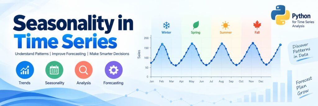
In simple terms, seasonality refers to repeated patterns or cycles in data that occur at consistent intervals, such as daily, weekly, monthly, quarterly, or annually. These patterns are often influenced by external, time-dependent factors, including:

• Weather changes
• Holidays and festivals
• Economic or fiscal cycles

Identifying these recurring fluctuations helps analysts distinguish regular changes from unusual behavior or outliers. For example, retail sales often increase during holiday seasons, while electricity consumption may rise during summer because of increased air-conditioning usage.

Characteristics of Seasonality

Several characteristics help define seasonality in time series data.

Repetition at Fixed Intervals

Seasonal patterns occur at consistent time intervals, such as every week, month, quarter, or year. This regularity makes them easier to recognize and incorporate into forecasting models.

Driven by External Influences

Seasonal behavior is commonly affected by external factors such as climate, cultural events, holidays, and industry-specific patterns.

Regular and Predictable

Unlike random fluctuations, seasonal variations generally follow a recurring rhythm. This predictability allows organizations to prepare for expected changes in demand or activity.

Why Seasonality Matters

1. Better Forecasting

Recognizing seasonal cycles can improve forecasting accuracy. For example, retailers can prepare inventory in advance of periods when festive shopping is expected to increase.

2. Optimal Resource Allocation

Anticipating increases or decreases in demand helps businesses manage employees, logistics, inventory, and other resources more efficiently.

3. Detecting Anomalies

Understanding normal seasonal behavior makes it easier to identify unusual changes. For example, a significant sales decline during a normally strong seasonal period could indicate an underlying business problem.

How to Identify Seasonality

Several analytical and visualization techniques can be used to identify seasonal patterns in time series data.

1. Visualization

Line charts and seasonal plots can make recurring patterns easier to recognize visually.

seasonal_plot(X, y='sales', period='week', freq='day')

2. Decomposition

Time series decomposition separates data into three major components: trend, seasonality, and residuals. This makes it easier to examine the contribution of each component.

STL (Seasonal and Trend decomposition using Loess) is one useful technique for separating these components.

3. Periodogram and Fourier Analysis

Periodograms and Fourier analysis transform time series data into the frequency domain, making it possible to identify dominant repeating frequencies and seasonal cycles.

plot_periodogram(average_sales)

4. Autocorrelation

Autocorrelation measures how strongly past observations are related to observations at different time lags. Peaks in an autocorrelation function (ACF) plot can indicate the presence of recurring seasonal patterns.

5. Seasonal Adjustment

Seasonal effects can be removed using statistical techniques such as STL or seasonal ARIMA. This allows analysts to focus more clearly on the underlying trend and other non-seasonal behavior.

Code Implementation: Detecting Seasonality in Store Sales

Let us implement a practical example using Python to analyze seasonal patterns in store sales data.

Import Libraries

import pandas as pd
import matplotlib.pyplot as plt
from pathlib import Path
from learntools.time_series.utils import plot_periodogram, seasonal_plot

Load Data

comp_dir = Path('../input/store-sales-time-series-forecasting')

sales_of_store = pd.read_csv(
    comp_dir / 'train.csv',
    usecols=['nbr_store', 'family', 'date', 'sales'],
    parse_dates=['date']
)

sales_of_store['date'] = sales_of_store.date.dt.to_period('D')

sales_of_store = (
    sales_of_store
    .set_index(['nbr_store', 'family', 'date'])
    .sort_index()
)

Analyze Seasonal Patterns

average_sales = (
    sales_of_store
    .groupby('date')
    .mean()
    .squeeze()
    .loc['2017']
)

X = average_sales.to_frame()

X["week"] = X.index.week
X["day"] = X.index.dayofweek

seasonal_plot(X, y='sales', period='week', freq='day')
plot_periodogram(average_sales)

The seasonal plot and periodogram can be used together to identify recurring patterns in the sales data. In this example, the analysis highlights weekly and biweekly seasonal behavior. The periodogram also indicates monthly components, which may be associated with recurring payment or wage-related purchasing patterns.

Modeling with Fourier Features

Fourier terms can be used to represent more complex seasonal cycles in a time series model.

from statsmodels.tsa.deterministic import CalendarFourier, DeterministicProcess

fourier = CalendarFourier(freq='W', order=4)

dp = DeterministicProcess(
    index=y.index,
    order=1,
    seasonal=False,
    additional_terms=[fourier],
    drop=True,
)

X = dp.in_sample()

X['NewYear'] = (
    X.index.dayofyear == 1
).astype('category')

Fourier features allow a model to represent repeating seasonal patterns using combinations of sine and cosine functions. They can be particularly useful when seasonal behavior is more complicated than a simple repeating indicator.

Visualizing Trend Over Time

Plotting the complete sales series can help reveal the overall trend and recurring variations.

sales_of_store.groupby('date').mean().squeeze().plot()

For a more detailed view, you can focus on a specific date range.

start_date_train = '2017-04-01'
valid_end_date = '2017-08-15'

sales_of_store.groupby('date').mean().squeeze().loc[
    start_date_train:valid_end_date
].plot()

Comparing Sales of Specific Items

You can also compare actual and predicted sales for a particular store and product category.

nbr_store = '1'
FAMILY = 'BEVERAGES'

ax = y.loc(axis=1)['sales', nbr_store, FAMILY].plot()

ax = y_pred.loc(axis=1)['sales', nbr_store, FAMILY].plot(ax=ax)

ax.set_title(f'{FAMILY} Sales at Store {nbr_store}')

Try different store numbers and product categories to understand how seasonal effects vary across locations and product families.

YT:- DecodeIT

Final Thoughts

Seasonality is more than just a statistical concept; it can be a valuable strategic asset. From improving inventory and pricing strategies to identifying unusual operational behavior, recognizing and modeling seasonal patterns can help businesses make smarter and more proactive decisions.

For anyone working with time series data, understanding seasonality is an essential skill. By combining visualization, decomposition, autocorrelation, periodograms, and Fourier features, analysts can better understand recurring patterns and incorporate them into forecasting models.

Keywords: seasonality in time series, seasonality in time series example, trend in time series, how to check seasonality in time series, seasonality in time series Python, types of seasonality in time series, cyclical seasonality in time series example, how to check seasonality in time series in R, how to check seasonality in time series in Excel, stationarity in time series, cyclical variation in time series