Logistic Regression in Machine Learning
Machine Learning plays a major role in today’s technology, especially when it comes to solving classification problems. One of the most widely used algorithms for classification is Logistic Regression.
Despite its name, Logistic Regression is not primarily a regression algorithm. It is a classification algorithm used to predict categorical outcomes such as Yes/No, Spam/Not Spam, or Cancerous/Not Cancerous.
In this guide, we will understand Logistic Regression, its working principle, sigmoid function, mathematical formula, types, assumptions, and a practical Python implementation.
Complete Advance AI Topics: Click Here
SQL Tutorial: Click Here
What is Logistic Regression?
Logistic Regression is a Supervised Learning algorithm mainly used for binary classification problems. Unlike Linear Regression, which predicts continuous numerical values, Logistic Regression predicts the probability of a categorical outcome.
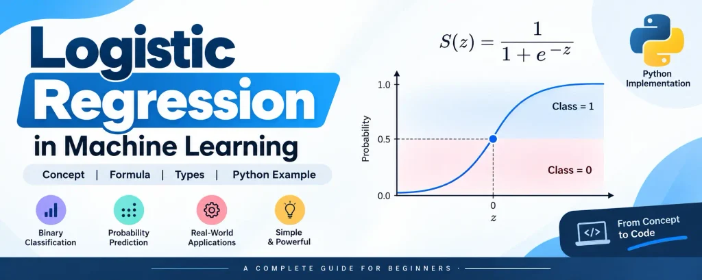
Instead of directly predicting values such as 0 or 1, Logistic Regression calculates a probability between 0 and 1. This probability is generated using a mathematical function called the Sigmoid Function, also known as the Logistic Function.
The predicted probability is then converted into a class using a threshold, commonly 0.5:
- If probability > 0.5, the predicted class is 1.
- If probability < 0.5, the predicted class is 0.
Why Use Logistic Regression?
- It provides a probabilistic interpretation of classification results.
- It can work with both discrete and continuous features.
- It provides useful insights into the contribution of input features.
- It is efficient, simple to implement, and widely used in real-world applications.
The Sigmoid (Logistic) Function
The Sigmoid Function is at the heart of Logistic Regression. It converts the output of a linear equation into a value between 0 and 1.
The sigmoid function is represented as:
S(z) = 1 / (1 + e-z)
Here, z represents the linear combination of the input features. Because the sigmoid function always produces an output between 0 and 1, its result can be interpreted as a probability.
Logistic Regression in Machine Learning – A Complete Guide
Image Source: Wikipedia – The classic S-shaped curve of the logistic function.
Logistic Regression Equation
Logistic Regression starts with a linear combination of the input variables, similar to Linear Regression:
z = b0 + b1x1 + b2x2 + … + bnxn
This value is then passed through the sigmoid function:
p = 1 / (1 + e-z)
For classification, Logistic Regression can also be expressed using the log-odds or logit function:
log(p / (1 – p)) = b0 + b1x1 + b2x2 + … + bnxn
This relationship allows the model to connect the input variables with the probability of belonging to a particular class.
Types of Logistic Regression
Binomial Logistic Regression
Used when there are two possible outcomes, such as Yes/No, 0/1, or Spam/Not Spam.
Multinomial Logistic Regression
Used when there are three or more unordered categories, such as Dog/Cat/Rabbit.
Ordinal Logistic Regression
Used when there are three or more ordered categories, such as Low/Medium/High.
Python Implementation: Predicting SUV Purchase
Let’s understand Logistic Regression with a practical Python example. In this example, we will use features such as Age and Estimated Salary to predict whether a customer will purchase an SUV.
Step 1: Data Preprocessing
import numpy as np
import pandas as pd
import matplotlib.pyplot as plt

# Load dataset
data_set = pd.read_csv('user_data.csv')

# Extract features (Age, Salary) and target (Purchased)
x = data_set.iloc[:, [2, 3]].values
y = data_set.iloc[:, 4].values
Step 2: Splitting the Dataset
Next, we divide the dataset into training and testing sets. Here, 25% of the data is used for testing.
from sklearn.model_selection import train_test_split

x_train, x_test, y_train, y_test = train_test_split(
    x, y, test_size=0.25, random_state=0
)
Step 3: Feature Scaling
Feature scaling helps bring the input features onto a similar scale, which can improve the learning process.
from sklearn.preprocessing import StandardScaler

sc = StandardScaler()

x_train = sc.fit_transform(x_train)
x_test = sc.transform(x_test)
Step 4: Fitting Logistic Regression
Now, we create the Logistic Regression classifier and train it using the training dataset.
from sklearn.linear_model import LogisticRegression

classifier = LogisticRegression(random_state=0)
classifier.fit(x_train, y_train)
Step 5: Predicting Test Set Results
After training the model, we use the test dataset to make predictions.
y_pred = classifier.predict(x_test)Step 6: Confusion Matrix
A Confusion Matrix helps evaluate the classification model by showing the predicted results compared with the actual results. It includes values such as True Positives, True Negatives, False Positives, and False Negatives.
from sklearn.metrics import confusion_matrix

cm = confusion_matrix(y_test, y_pred)

print("Confusion Matrix:\n", cm)
Step 7: Visualizing the Results
We can visualize the Logistic Regression model and its decision boundary using Matplotlib.
from matplotlib.colors import ListedColormap

x_set, y_set = x_train, y_train

x1, x2 = np.meshgrid(
    np.arange(
        start=x_set[:, 0].min() - 1,
        stop=x_set[:, 0].max() + 1,
        step=0.01
    ),
    np.arange(
        start=x_set[:, 1].min() - 1,
        stop=x_set[:, 1].max() + 1,
        step=0.01
    )
)

plt.contourf(
    x1,
    x2,
    classifier.predict(
        np.array([x1.ravel(), x2.ravel()]).T
    ).reshape(x1.shape),
    alpha=0.75,
    cmap=ListedColormap(('red', 'green'))
)

plt.xlim(x1.min(), x1.max())
plt.ylim(x2.min(), x2.max())

for i, j in enumerate(np.unique(y_set)):
    plt.scatter(
        x_set[y_set == j, 0],
        x_set[y_set == j, 1],
        c=ListedColormap(('red', 'green'))(i),
        label=j
    )

plt.title('Logistic Regression (Training set)')
plt.xlabel('Age')
plt.ylabel('Estimated Salary')
plt.legend()
plt.show()
The resulting visualization provides a clear representation of how Logistic Regression separates different classes using a decision boundary.
Assumptions of Logistic Regression
- The dependent variable should be categorical.
- There should be no significant multicollinearity among the independent variables.
- The log odds of the outcome should have a linear relationship with the independent variables.
Download New Real Time Projects :- Click here
Conclusion
Logistic Regression is a fundamental and powerful machine learning algorithm for classification problems. It can be used for applications such as email classification, disease prediction, customer behavior analysis, and many other real-world tasks.
Its simplicity, interpretability, efficiency, and probability-based predictions make it a popular choice when understanding the likelihood of an outcome is as important as making the final classification.
Pro Tip
Before moving to complex models such as Random Forests or Neural Networks, make sure you understand Logistic Regression well. A properly designed and tuned simple model can sometimes perform better than a complex model that has not been properly optimized.
Keywords: logistic regression in machine learning with example, logistic regression in machine learning python, logistic regression formula machine learning, linear regression in machine learning, logistic regression explained with example, logistic regression algorithm, logistic regression algorithm steps