Support Vector Machine Algorithm: Explained with Python Example

Support Vector Machine Algorithm

Machine Learning has transformed the way we analyze data and build intelligent systems. Among the many powerful algorithms used in Machine Learning, the Support Vector Machine (SVM) is one of the most effective choices for classification tasks.

SVM is a supervised learning algorithm primarily used for classification, although it can also be applied to regression problems. Its main strength is its ability to identify an optimal decision boundary between different classes, making it a reliable and versatile Machine Learning algorithm.

Complete Advance AI Topics: Click Here
SQL Tutorial: Click Here

What is SVM?

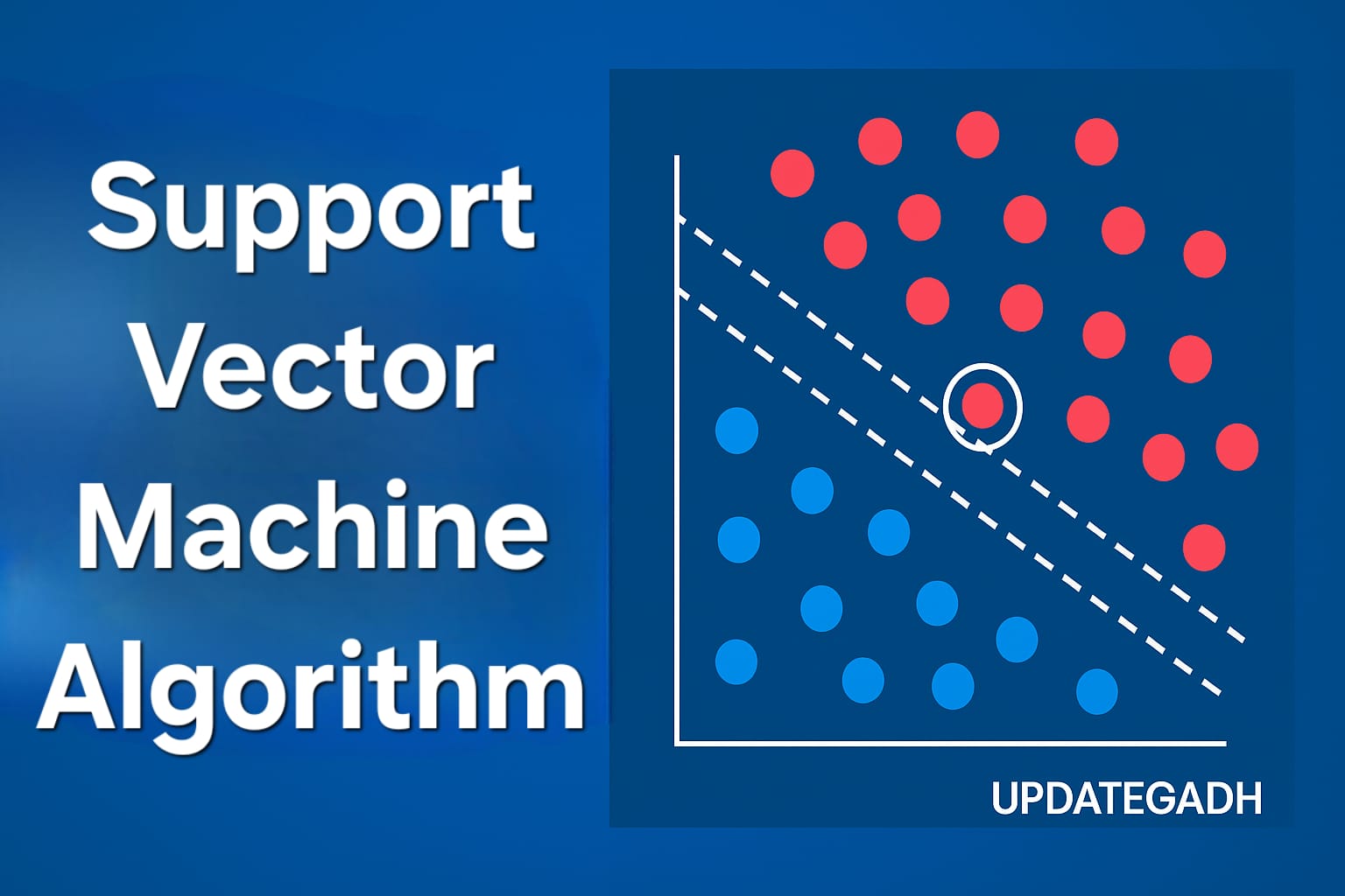
At its core, Support Vector Machine tries to find the best possible line, or hyperplane, that separates different classes in an n-dimensional feature space.

Once this decision boundary is determined, it can be used to classify new and unseen data points. But SVM does not simply choose any boundary that separates the classes. Instead, it looks for the boundary that provides the maximum margin between the classes.

The hyperplane is determined using specific data points called support vectors. These are the observations located closest to the decision boundary. They play an important role because they determine the position and orientation of the hyperplane.

This is where the name Support Vector Machine comes from.

SVM in Action: A Simple Example

Imagine that you are training a Machine Learning model to classify animals as either cats or dogs. You provide the model with many examples of both animals and allow it to learn their characteristics.

Now suppose the model receives a new image that contains features similar to both a cat and a dog. SVM uses the learned decision boundary and the important data points near that boundary to determine which class the new observation belongs to.

This approach makes SVM useful for several applications, including:

• Face Detection
• Image Classification
• Text Categorization

Types of SVM

Support Vector Machines can generally be divided into two main types:

1. Linear SVM

• Used when the data is linearly separable.
• The different classes can be separated using a straight line or hyperplane.

2. Non-Linear SVM

• Used when the data is not linearly separable.
• Uses kernel techniques to transform the data into a higher-dimensional space where the classes can be separated more effectively.

Download New Real Time Projects :- Click here

Hyperplane & Support Vectors

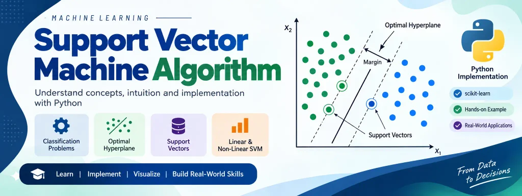
• Hyperplane: A decision boundary in the feature space that separates different classes.
• Support Vectors: The data points closest to the hyperplane. These points determine the position and orientation of the decision boundary.

SVM attempts to maximize the margin, which is the distance between the hyperplane and the closest support vectors from the different classes.

A larger margin generally helps the model generalize better when it encounters new data.

How Does SVM Work?

Linear SVM

Suppose we have two classes, green and blue, and two features, x1 and x2. There may be several possible lines capable of separating the two classes.

Instead of selecting an arbitrary line, SVM searches for the decision boundary that provides the maximum margin between the classes. This boundary is known as the optimal hyperplane.

Non-Linear SVM

Many real-world datasets cannot be separated using a simple straight line. In such situations, SVM can use a kernel function to transform the data into a higher-dimensional space.

For example, data that cannot be separated in two dimensions may become separable after being mapped into three dimensions.

One simple transformation can be represented as:

z = x² + y²

After transforming the data into a higher-dimensional space, a plane may be able to separate the classes. When this boundary is viewed in the original two-dimensional space, it can produce a non-linear boundary such as a circular decision region.

Implementing SVM in Python

Let’s now implement an SVM classifier using the popular scikit-learn library.

1. Data Pre-processing

import numpy as np
import matplotlib.pyplot as plt
import pandas as pd

# Importing dataset
dataset = pd.read_csv('user_data.csv')

# Extract features and labels
x = dataset.iloc[:, [2, 3]].values
y = dataset.iloc[:, 4].values

# Split into train and test sets
from sklearn.model_selection import train_test_split

x_train, x_test, y_train, y_test = train_test_split(
    x, y, test_size=0.25, random_state=0
)

# Feature scaling
from sklearn.preprocessing import StandardScaler

sc = StandardScaler()
x_train = sc.fit_transform(x_train)
x_test = sc.transform(x_test)

2. Fitting the SVM Classifier

from sklearn.svm import SVC

# Using a linear kernel
classifier = SVC(kernel='linear', random_state=0)

classifier.fit(x_train, y_train)

3. Making Predictions

# Predict test set results
y_pred = classifier.predict(x_test)

4. Evaluating with Confusion Matrix

from sklearn.metrics import confusion_matrix

cm = confusion_matrix(y_test, y_pred)

print(cm)

Output: The confusion matrix helps us understand how many predictions were classified correctly and incorrectly. A model with more correct predictions generally indicates better classification performance.

5. Visualizing the Results (Training Set)

from matplotlib.colors import ListedColormap

x_set, y_set = x_train, y_train

x1, x2 = np.meshgrid(
    np.arange(
        start=x_set[:, 0].min() - 1,
        stop=x_set[:, 0].max() + 1,
        step=0.01
    ),
    np.arange(
        start=x_set[:, 1].min() - 1,
        stop=x_set[:, 1].max() + 1,
        step=0.01
    )
)

plt.contourf(
    x1,
    x2,
    classifier.predict(
        np.array([x1.ravel(), x2.ravel()]).T
    ).reshape(x1.shape),
    alpha=0.75,
    cmap=ListedColormap(('red', 'green'))
)

plt.xlim(x1.min(), x1.max())
plt.ylim(x2.min(), x2.max())

for i, j in enumerate(np.unique(y_set)):
    plt.scatter(
        x_set[y_set == j, 0],
        x_set[y_set == j, 1],
        c=ListedColormap(('red', 'green'))(i),
        label=j
    )

plt.title('SVM (Training set)')
plt.xlabel('Age')
plt.ylabel('Estimated Salary')
plt.legend()
plt.show()

6. Visualizing the Results (Test Set)

x_set, y_set = x_test, y_test

# Similar visualization code as above

Conclusion

Support Vector Machines are powerful and reliable Machine Learning algorithms that can be used for both linear and non-linear classification problems. By maximizing the margin and concentrating on the most important boundary points, SVM can provide strong performance on many classification tasks.

Whether you are working with images, text, or structured datasets, SVM provides a mathematically sound approach for solving classification problems.

You can also experiment with different kernels such as linear, rbf, and poly, along with hyperparameters such as C and gamma, to improve the model’s performance for different datasets.

---

Keywords: Support Vector Machine Algorithm example, Support Vector Machine Algorithm machine learning, Support Vector Machine Algorithm pdf, hyperplane in Support Vector Machine Algorithm, svm solved example, support vector regression, linear svm, Support Vector Machine Algorithm, support vector machine algorithm in python, support vector machine algorithm example, support vector machine algorithm geeksforgeeks, svm algorithm in machine learning, support vector machine pdf, hyperplane in svm, svm algorithm steps