Gradient Descent in Machine Learning

Gradient Descent in Machine Learning

Gradient Descent is one of the most important optimization algorithms used in machine learning. From simple linear regression models to complex deep neural networks, gradient descent helps models reduce the difference between predicted and actual values. By repeatedly adjusting model parameters to minimize errors, it plays a key role in how many machine learning and AI systems learn from data.

In this blog post, we’ll explore what gradient descent is, how it works, the role of cost functions, the major types of gradient descent, and some of the common challenges associated with this optimization technique.

Complete Advance AI Topics: Click Here
SQL Tutorial: Click Here

What Is Gradient Descent?

Gradient Descent, also referred to as steepest descent, is an iterative optimization technique used to find the minimum value of a function. The method is commonly associated with the work of French mathematician Augustin-Louis Cauchy in the 19th century.

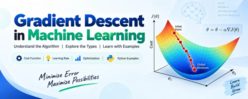
In machine learning, the main objective is often to minimize a cost function, which measures the difference between a model’s predicted outputs and the actual values. Gradient descent helps find a local minimum of this function by repeatedly moving in the direction opposite to the gradient.

Key Concept:

• Moving in the direction of the negative gradient helps minimize the function.
• Moving in the direction of the positive gradient increases the function and is known as Gradient Ascent.

The Role of Cost Functions

A cost function measures the difference between the expected and predicted values. It summarizes the model’s overall error into a single numerical value. During training, the objective is to reduce this error as much as possible.

Cost vs. Loss Function:

• A loss function measures the error for an individual training example.
• A cost function generally represents the average loss across the training dataset.

How Is It Used?

1. Start with an initial set of model parameters.
2. Calculate the value of the cost function.
3. Use gradient descent to adjust the parameters in a direction that reduces the error.
4. Repeat the process until the model reaches convergence or the cost stops improving significantly.

How Does Gradient Descent Work?

To understand how gradient descent works, consider the basic simple linear regression equation:

Y = mX + c

• m: Slope or weight
• c: Y-intercept or bias

The basic gradient descent workflow can be summarized as follows:

1. Start with initial values: Choose initial weights and biases, often randomly.
2. Calculate the gradient: Find the derivative of the cost function with respect to the model parameters.
3. Update the parameters: Adjust the weights and biases in the opposite direction of the gradient.
4. Repeat the process: Continue updating the parameters until the cost function reaches or approaches its minimum.

This repeated process allows a machine learning model to learn better parameter values from the available training data.

Learning Rate: The Step Size

The learning rate, commonly represented by α (alpha), determines the size of each step taken while updating the model parameters.

• A high learning rate can speed up training, but the algorithm may overshoot the minimum and fail to converge properly.
• A low learning rate can provide more controlled updates, but training may take much longer to reach convergence.

Choosing an appropriate learning rate is therefore important for achieving efficient and stable model training.

Types of Gradient Descent

Gradient descent is commonly divided into three main variants. Each approach has different advantages and trade-offs depending on the size of the dataset and the computational resources available.

1. Batch Gradient Descent (BGD)

In Batch Gradient Descent, the gradient is calculated using the entire training dataset before the model parameters are updated.

Advantages:

• Provides relatively stable convergence.
• Produces less noisy parameter updates.
• Works well with smaller datasets that can fit comfortably into memory.

2. Stochastic Gradient Descent (SGD)

Stochastic Gradient Descent updates the model parameters using one training example at a time.

Advantages:

• Works well with very large datasets.
• Requires less memory compared with processing the complete dataset for every update.
• The randomness in its updates can sometimes help the optimization process move away from problematic regions.

Trade-off: Because each update is based on a single training example, the optimization path can be noisy and may fluctuate around the minimum.

3. Mini-Batch Gradient Descent

Mini-Batch Gradient Descent combines ideas from Batch Gradient Descent and Stochastic Gradient Descent. Instead of processing the complete dataset or a single example, it uses a small batch of training examples for each update. Common batch sizes include 32, 64, or 128 samples.

Advantages:

• Combines the stability of Batch Gradient Descent with the speed of Stochastic Gradient Descent.
• Makes efficient use of computational resources.
• Often provides faster and more practical convergence during model training.

Common Challenges with Gradient Descent

Although gradient descent is widely used, it can face several challenges during optimization.

1. Local Minima and Saddle Points

• Local Minima: A point where the function has a lower value than the surrounding points, but it may not be the lowest value across the entire function.
• Saddle Point: A relatively flat point or region where the gradient can become very small, potentially slowing down the learning process even though the point is not a true minimum.

These situations can make optimization more difficult and may prevent the algorithm from reaching the best possible solution.

2. Vanishing and Exploding Gradients

Vanishing and exploding gradients are particularly important challenges when training deep neural networks.

• Vanishing Gradients: The gradients become extremely small, resulting in very small parameter updates. This can make learning difficult, especially in earlier layers of a deep network.
• Exploding Gradients: The gradients become extremely large, causing unstable parameter updates and potentially resulting in numerical problems such as NaN values.

Common solutions include:

• Batch normalization
• Gradient clipping
• Adaptive optimization algorithms such as Adam and RMSprop

Download New Real Time Projects :- Click here

Conclusion

Gradient descent is a foundational optimization technique in machine learning. It enables models to learn from training data by repeatedly adjusting their parameters to minimize prediction errors.

Whether you are developing a simple regression model or training a complex neural network, understanding gradient descent and selecting an appropriate variant can help you build more effective machine learning models.

Key Takeaways:

• Gradient descent minimizes a cost function by iteratively updating model parameters.
• The learning rate controls the size of each parameter update and is important for stable training.
• Batch, stochastic, and mini-batch gradient descent offer different approaches to model optimization.
• Local minima, saddle points, and unstable gradients can create challenges during training.

Stay tuned for more practical guides and detailed tutorials covering machine learning and AI fundamentals.

Keywords: gradient descent formula, gradient descent in neural network, gradient descent algorithm, stochastic gradient descent, gradient descent solved example, gradient descent in linear regression, gradient descent example, gradient descent meaning, gradient descent in machine learning with example, gradient descent in machine learning Python Machine LearningMachine Learning