Autocorrelation and Partial Autocorrelation
In the field of time series analysis, understanding how past observations influence future values is crucial for building accurate models and forecasts. Two core statistical tools that help uncover these relationships are autocorrelation and partial autocorrelation. These concepts not only shed light on patterns within data but also play a significant role in selecting the right time series models.
Machine Learning Tutorial:-Click Here
Data Science Tutorial:-Click Here
Complete Advance AI topics:-CLICK HERE
DBMS Tutorial:-CLICK HERE
What is Autocorrelation?
The association between a time series and its lagged variants over various time intervals is measured by autocorrelation, commonly referred to as serial correlation. In simple terms, it checks how the current value in a series relates to its previous values.
Key Aspects of Autocorrelation
- Definition: It refers to the correlation of a time series with its own past and future values at various lags.
- Positive Autocorrelation: Indicates that high values are likely to follow high values, and low values follow low ones—suggesting a trend or persistence in the data.
- Negative Autocorrelation: Suggests that high values are likely to be followed by low values and vice versa—indicating a reversal or oscillation pattern.
- Uses:
- Detecting trends and seasonal effects
- Identifying suitable lags in models like ARIMA
- Testing randomness in a dataset
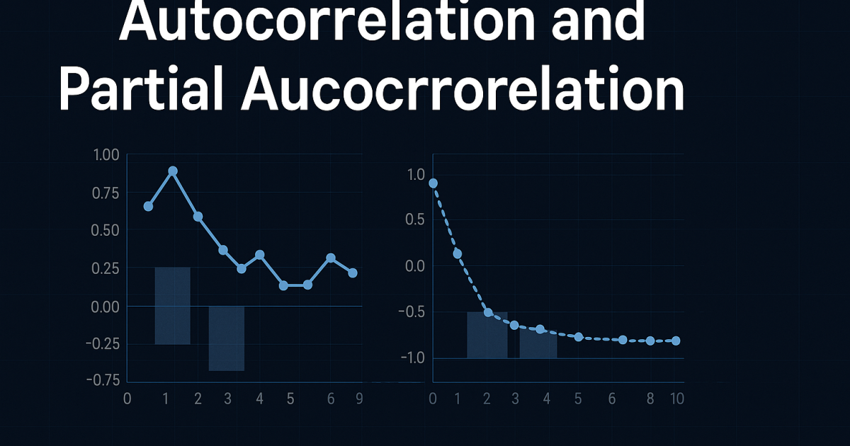
- Visualization: The Autocorrelation Function (ACF) plot displays autocorrelation coefficients at various lags, helping to identify recurring patterns.
Why is Autocorrelation Important?
In real-world scenarios, many time-dependent variables are influenced by their historical values. For instance, today’s stock price might be related to its performance over the past week. By measuring autocorrelation, analysts can detect such dependencies.
Ignoring autocorrelation in a time series can lead to misleading forecasts. For example, in linear regression applied to time-dependent data, not accounting for autocorrelation may result in biased coefficient estimates and unreliable inferences.
What is Partial Autocorrelation?
By eliminating the impact of intermediate lags, partial autocorrelation concentrates on the direct relationship between a time series and its lagged values.This concept is particularly useful for determining the appropriate number of lagged terms to include in an autoregressive model.
Key Aspects of Partial Autocorrelation
- Definition: Partial autocorrelation quantifies the direct impact of a lagged observation on the current value, isolating it from the effects of other lags.
- Uses:
- Ideal for selecting the correct order of an Autoregressive (AR) model
- Clarifies which lags have a direct effect, filtering out intermediate influence
- Visualization: The Partial Autocorrelation Function (PACF) plot shows the partial correlations at various lags, highlighting only significant direct relationships.
Why is Partial Autocorrelation Important?
Partial autocorrelation is essential for model identification in autoregressive processes. SIf a PACF plot reveals notable spikes at lags 1 and 2, but not beyond, this may indicate that an AR(2) model is suitable.In this case, the present value is directly influenced only by the previous two observations.
Autocorrelation vs. Partial Autocorrelation
Despite being essential instruments in time series analysis, autocorrelation and partial autocorrelation provide different perspectives:
| Feature | Autocorrelation | Partial Autocorrelation |
|---|---|---|
| Definition | Measures the total correlation between current and lagged values | Measures the direct correlation after removing effects of shorter lags |
| Purpose | Detects patterns like seasonality and trends | Identifies how many past values directly influence the present |
| Interpretation | High values may include indirect effects through intermediate lags | High values represent only the direct relationship |
| Model Use | Helps determine if differencing is needed or if MA terms are required | Helps decide the order of AR terms |
| Plot Type | ACF Plot | PACF Plot |
| Example | ACF at lag 2 includes influence of lag 1 | PACF at lag 2 removes influence of lag 1 |
Visualizing ACF and PACF
Plotting ACF and PACF is a standard practice in exploratory time series analysis:
- ACF Plot: Useful for detecting long-term trends, seasonality, or identifying if differencing is needed. A slowly decaying ACF plot indicates non-stationarity.
- PACF Plot: Helps determine the number of autoregressive terms. For example, if only lag 1 shows a significant spike, an AR(1) model might be sufficient.
Example Use Case
Imagine analyzing daily temperatures. The ACF might show strong correlations at lags 1 to 7 due to weekly patterns, whereas the PACF might show a significant spike only at lag 1, suggesting a direct one-day lag effect.
Complete Python Course with Advance topics:-Click Here
SQL Tutorial :–Click Here
Download New Real Time Projects :–Click here
Conclusion
Autocorrelation and partial autocorrelation are cornerstone techniques in time series modeling. Understanding them is critical for identifying patterns, selecting the correct model structure, and making reliable forecasts. Whether you’re working with financial data, climate statistics, or web traffic logs, mastering ACF and PACF helps unlock deeper insights and build better predictive models.
At Updategadh, we believe strong fundamentals are the key to advanced analytics. Stay tuned for more guides on time series modeling, forecasting techniques, and data-driven decision-making.
autocorrelation and partial autocorrelation in time series
partial autocorrelation formula
partial autocorrelation function
partial autocorrelation example
partial autocorrelation python
how to interpret partial autocorrelation plot
how to interpret autocorrelation plot
acf vs pacf
partial autocorrelation
difference between autocorrelation and partial autocorrelation
autocorrelation and partial autocorrelation formula
autocorrelation and partial autocorrelation example
🎓 Need Complete Final Year Project?
Get Source Code + Report + PPT + Viva Questions (Instant Access)
🛒 Visit UpdateGadh Store →